
Introduction to Darfix (2.x)#
darfix is a Python library for the analysis of dark-field microscopy data. It provides a series of computer vision techniques, together with a graphical user interface and an Orange3 (biolab/orange3) add-on. darfix is to be used as a workflow, where every step of the analysis can be applied independently. The aim of this tutorial is to guide you into correctly executing darfix into a correct analysis of your images.
The main functionalities of darfix can be divided in 3 parts:
Load the data and select the different motors (dimensions). Select a transformation technique (RSM, magnification), if needed.
Pre-analysis of the images by applying several operations like region of interest, noise removal and shift correction.
Apply DFXM analysis to the images. The DFXM techniques currently in darfix are:
Rocking curve imaging: The data is fitted along the z-dimension (pixel by pixel), to follow a certain distribution (gaussian). After that 3 maps are shown: intensity, FWHM, and … The fitted data is saved on disk in HDF5 format.
Grain plot: Several maps are plotted which can be exported into a single file: COM, FWHM, skewness, kurtosis (for every dimension), and mosaicity and orientation distribution maps in case of 2D datasets.
Blind source separation: An experimental technique that uses different blind source separation techniques to find grains along the dataset, tests with different datasets have shown good results with techniques like NMF, NNICA, and NMF+NNICA.
darfix can be either executed using plain code (using for example a jupyter notebook), or by using the Orange3 software that allows the creation of workflows in a GUI environment. This last is recommended in most cases as it allows for an easier and graphical view of the different steps. Once a workflow is created via Orange it can be saved and transformed to a single script using ewoks, which can then be executed with different dataset inputs. For now, to use darfix the dataset has to be of a certain format as the obtained scans from BM03:
The data format should either HDF5 or EDF
- Motor information should be contained in metadata.
For HDF5: a group should contain all positioners datasets.
for EDF: headers should contain motors_mne information.
The data should be images.
This tutorial will basically introduce the graphical interface using Orange, for a tutorial using the core functions of darfix you can go to darfix_tutorial.ipynb
How to access it#
If you have access to the slurm cluster (or any official esrf computer) you can use ‘linux’ modules to access the software. Else you will need to install it before using it.
With access to the ESRF cluster#
connect to the cluster
ssh -XC cluster-access
allocate node with appropriate resources
salloc -p interactive –x11 srun –pty bash
load the darfix module
module load darfix
Hint
you can specify a version to be used when loading darfix(module load darfix{version}). For example to load the ‘dev’ version:
module load darfix/dev
You can also use ml as an alias of module load
ml darfix
Launch darfix
darfix-canvas
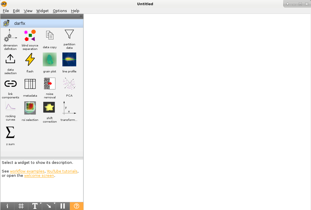
then the following window should appear:
without access to the ESRF cluster#
see Installation
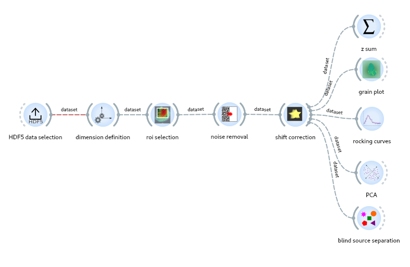
Workflow creation#
To create the workflow just click on any widget you want from the left (usually start with data selection). From every widget you can create links to other widgets:
Data selection#
Data selection can be done either from HDF5 or EDF datasets (legacy).
For a HDF5 dataset#
TODO:
For more details see HDF5 data selection
For a EDF dataset#
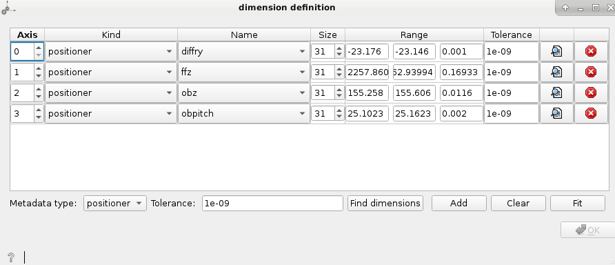
Dimension definition#
This step allows you to input the necessary motor information of the dataset, which will be used at future steps. Normally, you’ll want to set the dimensions to be the moving motors, for this the metadata type has to be set to positioner. The Find dimensions option will look for moving motors and show you the ones that change through the dataset (difference higher than the tolerance value). Once the dimensions are found, you can check which motors you want to work with and make sure the range values are ok. In case the minimum and maximum values are ok, but the step is wrong, you can set the step value to 0 and add the correct size.
After that you can try to Fit the dimensions. If the fit was correctly done it means that the product of the size of your motors corresponds to the number of images on your dataset. If the fit can’t be done look again at the range and size values.
Transformation#
The Transformation widget allows you to modify the axes of the plots so that they include the size in microns of the camera instead of the size in pixels. With one dimension datasets you can choose between a RSM transformation or a magnification. With two or more dimensions you can only apply magnification.
Partition#
In cases with a large number of images you may want to omit the images with low intensity. This widget allows you to see an intensity curve of the images and to choose how many images you want to keep. At the next steps of the workflow only the images with higher intensity will be used for the analysis.
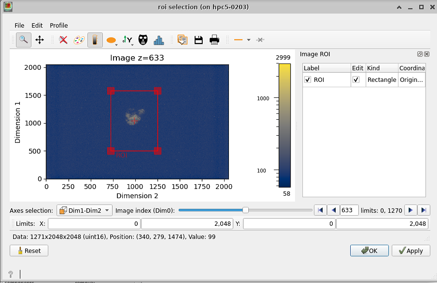
Region of interest#
If your sample appears only in a part of the image all along the dataset it’s good to apply a region of interest, both to make the analysis faster (less data), and to help you see closer the different features of the sample.
To select the ROI in the widget, you can move and reshape the red rectangle that appears on the view, and click Apply to see how the region will be applied. If the ROI is good for you, you can click OK to go to the next step. Apply has to be clicked before Ok for the ROI to be applied.
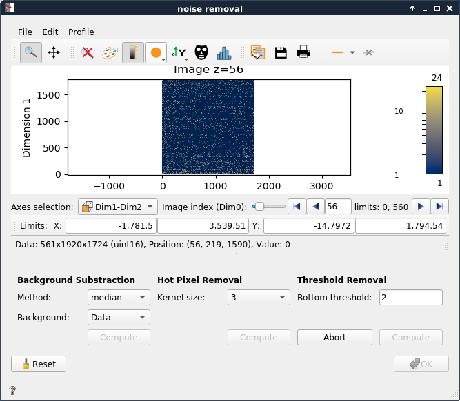
Noise removal#
This step allows you to subtract background and remove hot pixels and data below a certain threshold (user defined). If possible (specially when the data is not in memory) an Abort button will appear after clicking Compute (for each method), this allows to cancel the operation if needed.
Once you have completed noise removal you can press OK and follow to the next step of the procedure.
Tip
Consider the data! If the data/Background Intensity relation is big, you can considerably increase your threshold, if the difference between data and background is not so big, you might be losing information by removing too much.
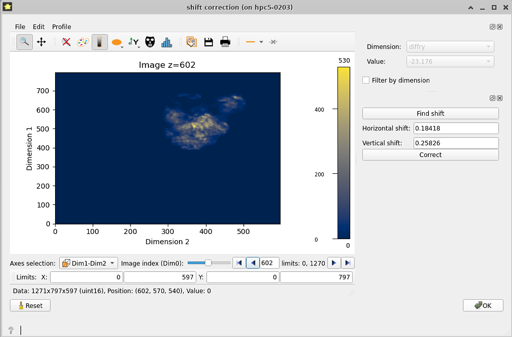
Shift detection and correction#
Depending on the acquisition conditions of the raw data, the consecutive images might show a displacement of the object of study that does not correspond to reality. This displacement is here identified as shift and can be calculated by the program. This can be done either simultaneously along all the dataset, or individually for each motor.
This last case is activated when clicking the Filter by dimension option. With this option active, the Find shift button loops through the values of the selected dimensions and finds, for each value, the linear shift of its corresponding images (the images that have that motor value, which are the ones you see on the plot). It not only finds the shift for the selected value but for all values of that dimension.
After the shift is found, you can move through the values and see the different found shifts. After that clicking Apply shift will apply all the shifts found to the corresponding images (although clicking Apply only to selected values, which only applies the shift to the images you see on the plot).
This step allows you to subtract background and remove hot pixels and data below a certain threshold (user defined).
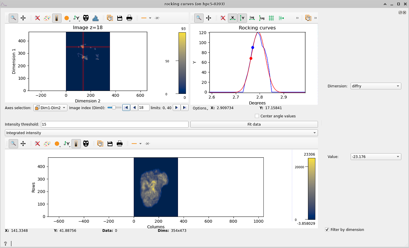
Rocking curve imaging#
The rocking curves widget allows you to see a curve of the intensity of each pixel along the dataset. The plot on the top left shows you the stack of images that you can move along. When clicking at any pixel on the plot, two curves will show on the top right plot, The blue curve is the rocking curve of the pixels intensity, and the red curve shows the rocking curves fit along a gaussian function.
If you are working with multi-motor datasets you’ll see that the rocking curve has many peaks, which results in a wrong fit curve. This is because there is a peak for each motor value. In such cases, you have to click on Filter by dimension and choose a motor and a value to work with.
Below the plots you have a button Fit data and a slot to enter an Intensity threshold. Clicking the button will fit all the pixels to a gaussian (it will compute the red curve for all the pixels of the image). The intensity threshold is used to fasten the computation by omitting pixels whose curve has no intensity variation: the entered number is the maximum intensity variation used to omit that pixel, above that the pixel will be fitted. With multi-motor datasets the fit will be recursively done along the chosen dimension values.
When the fitting has finished (it may take a while, you can see the progress on the terminal), four maps appear at the bottom: integrated intensity, FWHM, peak position and residuals map. These maps are computed using the fitted data and the residuals map is a measure of how good the fit is.
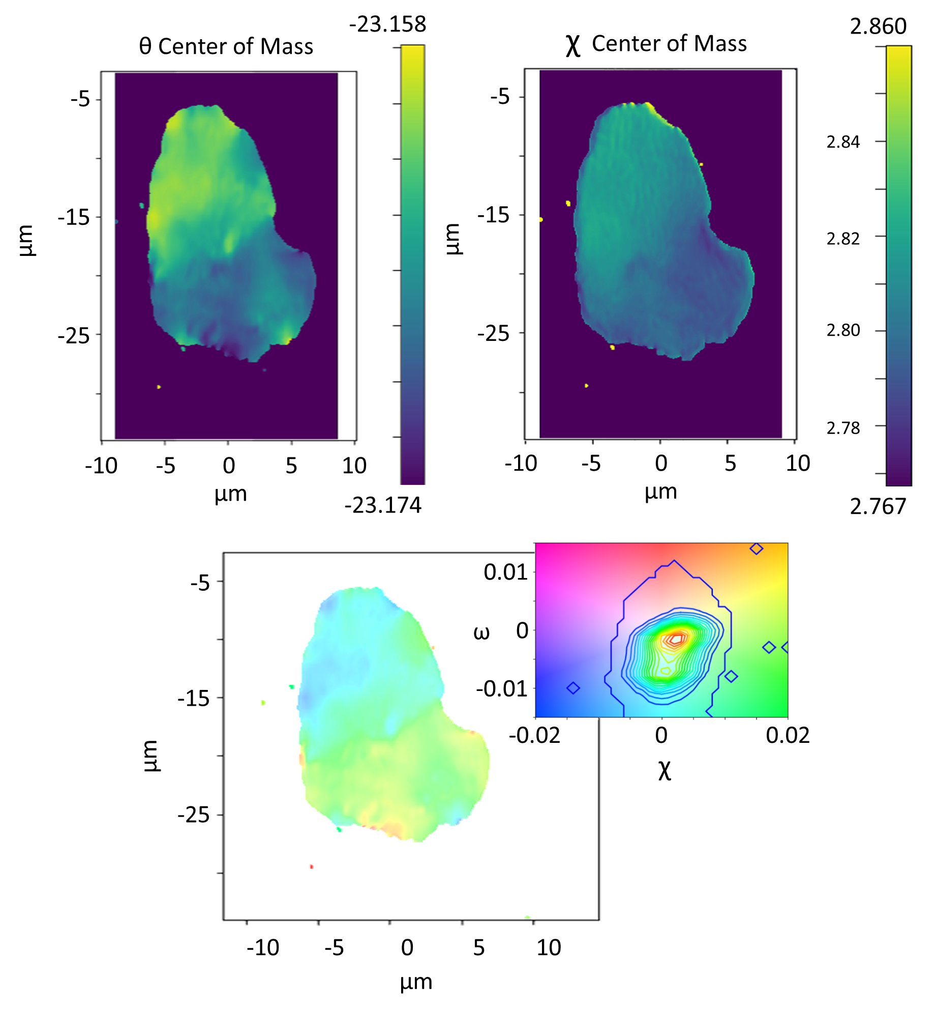
Grain plot#
Statistical measures can also be obtained by using the grain plot widget. This widget shows 6 maps:
Center of mass: Shows the COM map for every motor. The center of mass looks at the intensity as a function of a motor position, using the intensity values of the images as a statistical weight
FWHM, Skewness and Kurtosis: Full width half maximum map, same as COM but with the standard deviation, skewness and kurtosis.
Mosaicity: the mosaicity map is an hsv image that has the COM of the first motor as hue and the COM of the second motor as saturation.
Orientation distribution: hsv map key that works as a colormap for the mosaicity and that includes the contour map of the orientation distribution.
Blind Source Separation#
Blind source separation (BSS) comprises all techniques that try to decouple a set of source signals from a set of mixed signals with unknown (or very little) information. darfix includes some BSS techniques to try to find the different grains along the dataset.
But first, the number of components has to be estimated, it can either be done automatically by clicking the Detect number of components button, or using the PCA widget.
This widget uses the technique of principal components analysis to find the singular values with more intensity:

Note
in this example we would take 4 or 5 components.
When automatically detecting the number of components, darfix uses the same technique with PCA, and takes the components that represent the 99% of the dataset.
The Blind source separation widget includes different techniques to find the components: Principal components analysis (PCA), non-negative independent component analysis (NICA) and non-negative matrix factorization (NMF).
Although the first one is available for use, it is not recommended since PCA doesn’t take into account the positivity of the images, and doesn’t give good results.
NICA, although returning positive components, can give negative value at the weight values, and is usually also discarded. NMF on the other hand gives positive values for both components and weights, but as the decomposition matrices are randomly initialized, the result is non-unique.
To solve this last problem, we have a fourth method: NICA+NMF that uses the output of NICA as input for NMF. The final result is unique and is preferable to NMF alone, although it is a bit slower.
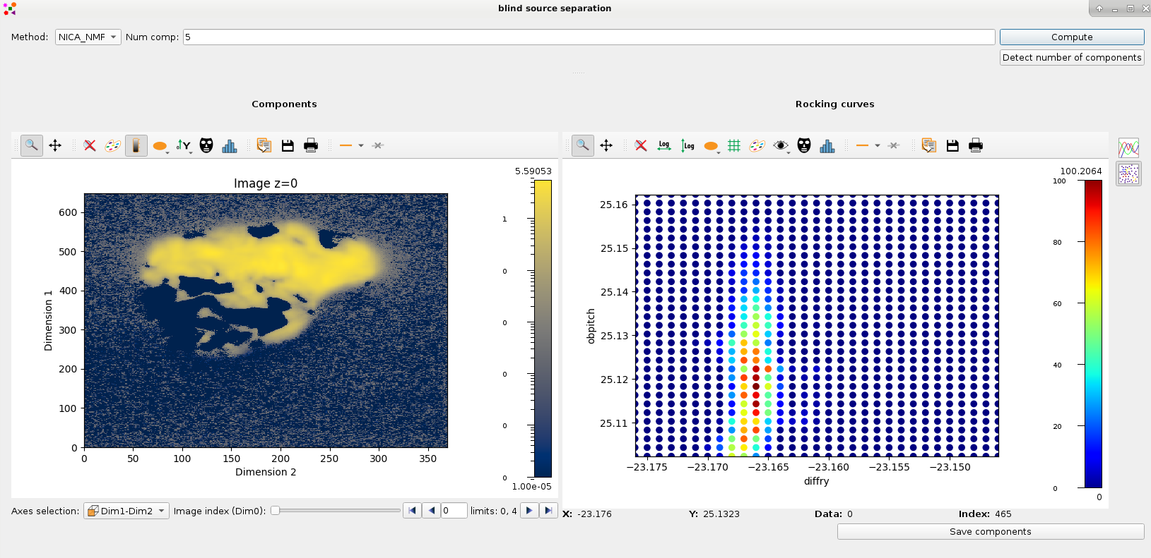
Once computed, the components can be seen on the left plot, while on the right we have different plots of the weights values.
At the right of the widget we can choose to either see the weights in terms of rocking curves, or see them in terms of an RSM map (like in the figure). Either way, these plots serve useful to see how each component is present in the dataset.
For the RSM, changing the component on the left changes its RSM map on the right.
After the analysis is done, you can save the components into an hdf5 file by clicking at the Save components button.
TODO: link components, flash, batch processing, partition data.